Transformation Matrices – Direct 2D Translations

Transformation Matrices – Direct 2D Translations

In this series I’m going to do my best to demystify something that has terrorfied and confused me for several years until a great collogue of mine Catarina Carvalheiras sat me down and put it terms that my brain could understand so I’m going to do my best to re-explain it in the same manor. To start of were going to concentrate on Direct 2D translations only.

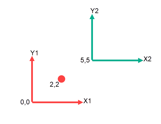
What does direct mean? Imagine you have an axis system at 0,0 and a point constructed from that axis system at 2,2. We now add another axis system at 5,5 where is the point in respect to the second axis system. Its like two people looking at a ball in a room, the ball isn’t moving but its position in respect to each person is at a different location. The caveat to this is the first person is sat in the corner of the room at 0,0,0 and knows where the second person is sitting in terms of X,Y,Z.

We can easily look at the problem and say that the point in respect to the second axis system is -3,-3 and this is true since the first axis system in respect to the second axis system is -5,-5 + the points location in respect to the first axis system 2,2. So we can do the math -5+2, -5+2 = -3,-3.

But we should be able to do this in a more mathematical manor.

So the first general equation is shown below which says the Point in respect to reference frame 1 is equal to the transformation matrix multiplied by the point in respect to the original reference frame. Here we also show the matrix dimensions and we can see that we can not multiply the point in respect to the original reference frame by the transformation matrix.

\begin{gather*}

P|_1 = [T] \cdot P|_0 \\

\begin{bmatrix}
   x_1 \\
   y_1 \\
   1
\end{bmatrix} 
= \begin{bmatrix}
   t_{11} &   t_{12} & t_{13} \\
   t_{21} &   t_{22} & t_{23} \\
   0 &   0 & 1 \\
\end{bmatrix}
\cdot
\begin{bmatrix}
   x_0 \\
   y_0 \\
   1
\end{bmatrix} \\
\lbrack 3 \times1 \rbrack = \lbrack 3 \times3 \rbrack \cdot  \lbrack 3 \times 1 \rbrack

\end{gather*}

The general form of the transformation matrix is as follows, Rotational matrix ‘[R]’ Rotation matrix multiplied by the Position matrix ‘[R].[P]’, as many 0’s as required, and a 1.

T_{xy} =\begin{vmatrix}
   \lbrack R \rbrack  & \lbrack R \rbrack \cdot\lbrack P \rbrack \\
   0... & 1
\end{vmatrix}

Since we are only dealing with Position for this conversation it simplifies our transformation matrix to:

T_{xy} = \begin{vmatrix}
   \lbrack R \rbrack  & \lbrack P \rbrack \\
   0... & 1
\end{vmatrix}

We can see that our matrix has matrices inside [R] and [P], so lets look at the expanded form of ‘[R]’ the rotational matrix which will be identity but lets see how that’s derived.

We have to look at vectors X2 and Y2 in respect to the original reference frame, since there are no rotations these will be:

\begin{align*}
\overrightarrow{X2} = {1\brack 0} \\
\overrightarrow{Y2} = {0\brack 1} \\
\end{align*}

We can now expand out our transformation matrix to:

T_{xy} = \begin{vmatrix}
    1 & 0 & \lbrack P \rbrack \\
    0 & 1 \\
    0 & 0 & 1
\end{vmatrix}

Which now only leaves the [P] position matrix. since we have to look at the position from the new reference frame back to the original reference frame. We know that the new reference frame was offset by 5,5. What were really saying is the position of the new reference frame in respect to the original reference frame is 5,5. However we we need to look the other way the original reference frame in respect to the new reference frame, which will be -5,-5, we can simply multiple the two values by -1. If we populate the matrix with these two values we will get;

T_{xy} = \begin{vmatrix}
    1 & 0 & -5 \\
    0 & 1 & -5\\
    0 & 0 & 1
\end{vmatrix}

We can now go ahead and do the calculation to see where the point is in respect to the new reference frame.

\begin{gather*}
P|_1 = [T] \cdot P|_0 \\

\begin{bmatrix}
   x_1 \\
   y_1 \\
   1
\end{bmatrix} 
= \begin{bmatrix}
   1 & 0 & -5 \\
   0 & 1 & -5  \\
   0 & 0 & 1 \\
\end{bmatrix}
\cdot
\begin{bmatrix}
   2 \\
   2 \\
   1
\end{bmatrix} \\

\begin{equation*}
\begin{split}
x_1= (1*2) + (0*2) + (-5*1) \\
x_1= 2 + 0 + (-5) \\
\bold{x_1= -3}\\
y_1 = (0*2) + (1*2) + (-5*1) \\
y_1 = 0 + 2 + (-5) \\
\bold{y_1 = -3}\\
1 = (0*2) + (0*5) + (1*1) \\
1= 0 + 0 + 1 \\
\bold{1=1}
\end{split}
\end{equation*}

\end{gather*}

So now we have the transformation matrix we can plug in any point in respect to the original reference frame and understand where it is in respect to the new reference frame. So lets try a point at -3,4 in the context of the original reference frame.

We can do the math quickly by (-5 + -3) , (-5 + 4) = -8, -1

\begin{gather*}
P|_1 = [T] \cdot P|_0 \\

\begin{bmatrix}
   x_1 \\
   y_1 \\
   1
\end{bmatrix} 
= \begin{bmatrix}
   1 & 0 & -5 \\
   0 & 1 & -5  \\
   0 & 0 & 1 \\
\end{bmatrix}
\cdot
\begin{bmatrix}
   -3 \\
   4 \\
   1
\end{bmatrix} \\

\begin{equation*}
\begin{split}
x_1= (1*-3) + (0*4) + (-5*1) \\
x_1= (-3) + 0 + (-5) \\
\bold{x_1= -8}\\
y_1 = (0*-3) + (1*4) + (-5*1) \\
y_1 = 0 + 4 + (-5) \\
\bold{y_1 = -1}\\
1 = (0*-3) + (0*4) + (1*1) \\
1= 0 + 0 + 1 \\
\bold{1=1}
\end{split}
\end{equation*}

\end{gather*}

It works… 🙂