Basic Calculus

Basic Calculus

Let me start of by saying I’m a CAD freak and those who know me might be a little surprised by this post, but there are aspects of the CAD system that require some calculus and this is my goal and by creating these posts I’m aiming at teaching myself and maybe at the same time helping others. So I look forward to any comments on this subject.

We will look at integrals which help us find areas and volumes and derivatives which help us find the slope of a curve at a given point.

Integrals

So we have a curve that has a function f(x) = X^2 and we want to find the area under the curve between X= 4 and X=7 how do we do this?

First we have to write the integral, remember we raise the power by 1 and divide by the result of raising the power, in this case I’m assuming mm;

Area = \int_{4}^7 x^{2}dx \\
=\int_{4}^7x^{3}/3 \\
So \\
= (7^{3}/3 ) - (4^{3}/3 ) \\
= 114.333 - 21.333 \\
= 93mm^{2} \\

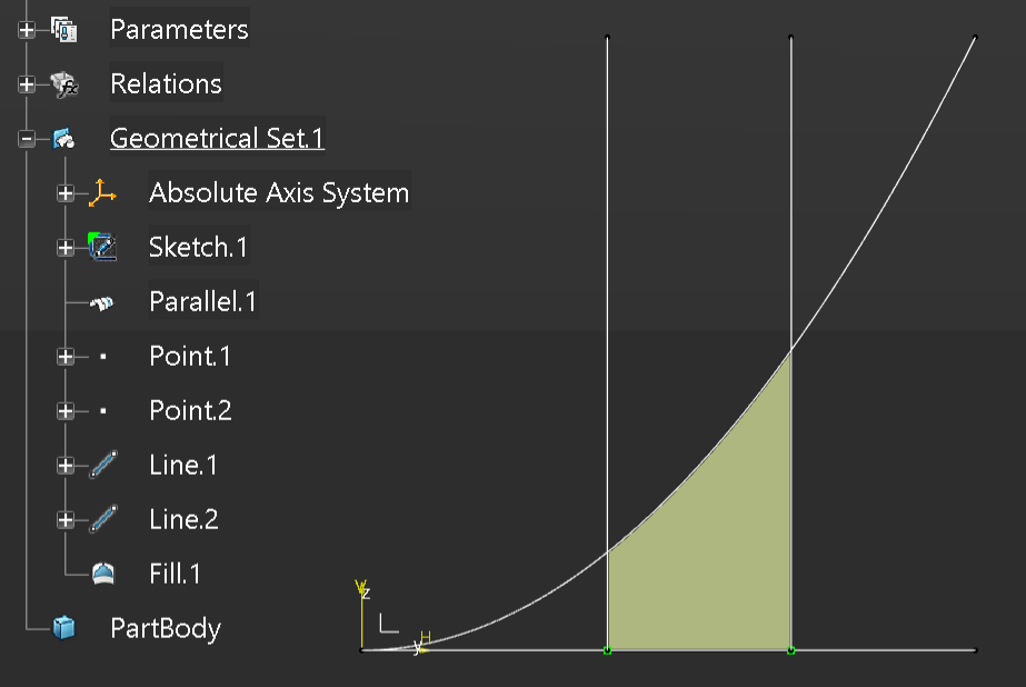
Let’ see this in action within a CAD model;

To do this we will create a Law where Y=X^2.

Notice that we multiply the result by 1000 to scale up the curve, since X is evaluated from 0 to 1.

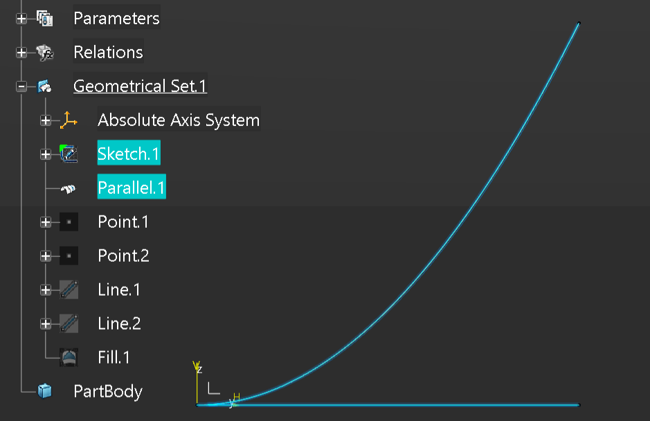
Then we will create a sketch that contains a horizontal line 1000mm long, then from this create a parallel curve that uses the law previously defined.

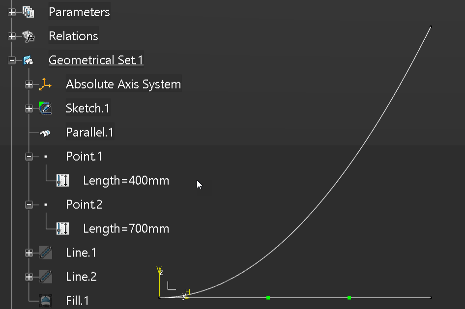
Next we will add two points on the horizontal line at 400mm and 700mm from the origin.

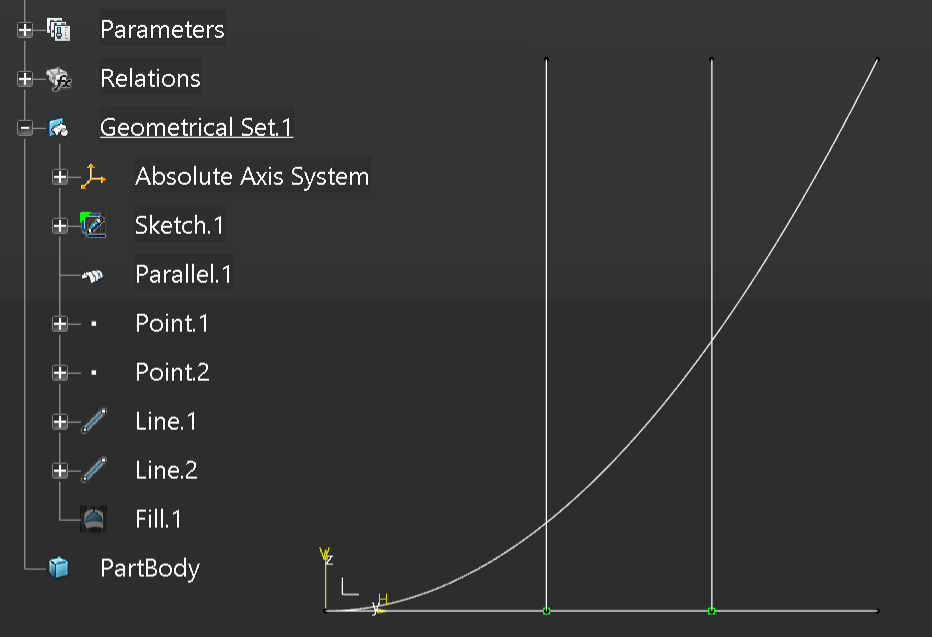
Next we will create two vertical lines 1000mm long from each of the two points.

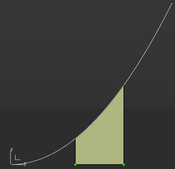
Finally a fill surface can be created to represent the area under the curve.

Now we will add an Area parameter and add the following formula to the parameter.

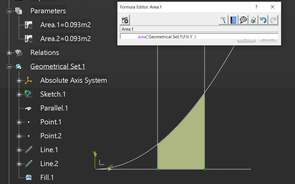
And finally we can use the equation we derived earlier.

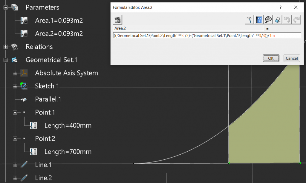
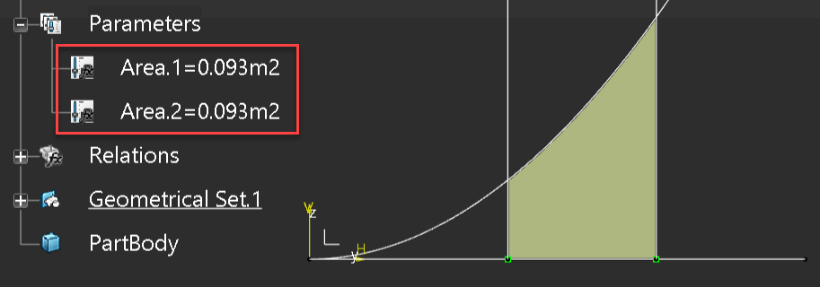
So we now have an exact comparison between what was measured and what was calculated by our equation, cool.

Point On Curve

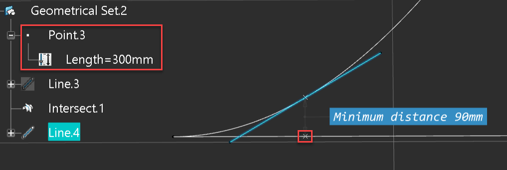
So we know the function of the curve f(x) = X^2, actually we have f(x) = X^2 *1000 and we have to remember this. We want to create a point by coordinated that always intersects the curve.

We know that the curve is on the YZ plane in the CAD system, therefor X = 0mm , we will give Y an arbitrary value 300mm and to calculate Z well use the following equation;

We can see that the point lays on the curve, but notice in the equation we had to divide by 1m (one meter) since we squared the Y value and the original law was scaled by 1000. So this means that we can do a little more math to determine the slope of the curve at a given point.

Derivatives

So we have a curve that has a function f(x) = X^2 and we want to find a tangent line for a given X value, in this case we have a given X value of 300 and a Y value of 90, this is where we use Derivatives.

The first thing we have to do is calculate the Y value, remembering the division by 1000;

f(x) = x^{2} / 1000\\
f(300) = 300^{2} / 1000\\
f(300) = 90,000 / 1000 \\
Y = 90

Next step is to determine F-Prime of X f'(x)

f'(x) = 2x^{1} \\
f'(x) = 2x \\

Next well plug in our X coordinate into f'(x) which defines our slope number

f'(x) = 2x / 1000 \\
f'(300) = 2 \cdot 300 / 1000 \\
f'(300) = 600 /1000 \\
f'(300) = 0.6

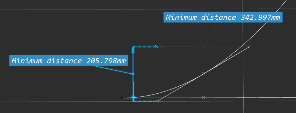
And we can prove this in the CAD model, if we draw a tangent line through the point on the curve, and then divide the rise by the run;

( 205.798mm / 342.997mm ) / 1000 = 0.599999 \\
\approxeq 0.6

The last step is to use the point slope formula for a line.

Y-Y_1 = M(X-X_1) \\
Y-90 = 0.6(X-300) \\
Y-90 = 0.6X - 180 \\
Y = 0.6X -180 + 90 \\
Y = 0.6X - 90\\

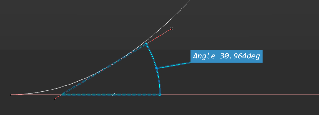
Since we know the slope number 0.6 we can calculate the Angle. To do this we will create a right angled triangle based on the slope number and do some simple trigonometry to determine the angle;

Run = 10mm \\
Rise = 10 * 0.6 = 6mm \\
Hypotenuse = \sqrt{ 10^2 + 6^2} \\
Hypotenuse  = 11.6619mm \\
Angle = Cos^{- 1}(10mm/11.6619mm) \\
Angle = 31.021 degrees

And here we have the the CAD representation of the angle.

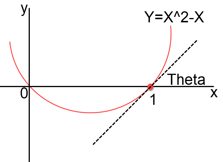
But the story is not over yet, there is a simpler way to calculate the angle, otherwise known as the angle Of Inclination. Let’s assume we have the following curve, and we want to determine the angle Theta;

Just as before we would determine F-Prime of X f'(x), remembering the rules;

• Power Rule – We Multiple the X by the power and then subtract 1 from the power so X^3 = 3X^2 and 2X^3 = 6X^2 notice in this case we multiplied out the X value.
• Line Rule – We remove the variable so 1X = 1

So let’s apply this to our problem;

f'(x) = x^{2}-x \\
which \enspace is \enspace really; \\
f'(x) = 1x^{2}-1x \\
f'(x) = 2x^{1} -1 \\
f'(x) = 2x -1 \\

So now we have the derivative we calculate the slope angle M by substituting X by 1

f'(x) = 2x -1 \\
f'(1) = 2\cdot1 -1 \\
f'(1) = 1 \\

If we use Trigonometry we have the Rise and Run but not the hypotenuse, so we must use the Opposite / Adjacent = Tan

and

we know that the Slope M = Rise/Run

which is equivalent to Tanθ = Rise/Run

which is equivalent to M = Tanθ

so

θ = Tan^-1M

Now we have the equation we can calculate the slope angle for an M value of 1;

θ = Tan^{-1}M \\
θ = Tan^{-1}\cdot1 \\
θ = 45\degree

And if we go back to our previous example where we had a slope angle for an M value of 0.6;

θ = Tan^{-1}M \\
θ = Tan^{-1}\cdot 0.6\\
 = 30.9637\degree

Which matches our CAD model exactly.